Originally posted on RViews
One of the most valuable things I have learned working on Data for Democracy’s Medicare drug spending project has been the value of collaborative tools. It has been my first in-depth experience using Github collaboratively, for one, but it has also introduced me to data.world.
data.world is an intuitive way to store, organize, explore, and visualize individual data files, making them more visible to and usable for anyone who’s interested. Using the data.world R package, I was able to collect the data I needed for one dashboard, create and publish a derived dataset, and build a Shiny dashboard that pulls live data from the site — all with complete visibility to my D4D teammates, who can now directly and easily access both the original and derived datasets.
The Beginning
Back in December, I started seeing posts about Data for Democracy floating around, and the idea immediately piqued my interest. I joined up not knowing what I would be doing exactly.
One of the ideas among pilot projects suggested by D4D leader Jonathon Morgan was looking at Medicare spending. Specifically, starting with the prescription spending data for 2011–2015 released by the Centers for Medicare and Medicaid Services. Out of all the original project ideas (check out the current and growing list of projects and be amazed), this one was most in my wheelhouse, and I jumped into the discussions to see what might happen.
D4D started developing some leadership structure, and Matt Gawarecki and I were asked to lead the drug spending project. We began by tidying the Medicare Part D spending data available from CMS.gov, which was straightforward enough (thanks, CMS!), and initially stored all that on our Github repo.
Soon, our A+ team of volunteers found data on therapeutic classes, lobbying expenditures, manufacturers, and more. As we looked for a better place to store and collaborate on our datasets, D4D projects started to leverage data.world. We decided that data.world was a good place for our data, too.
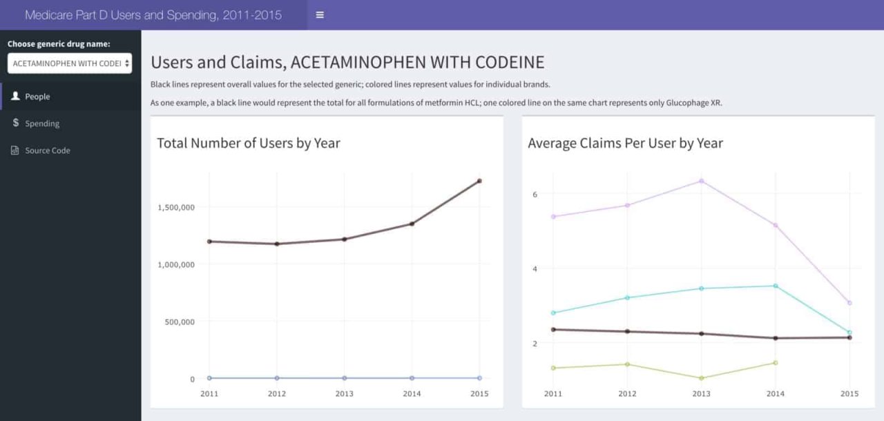
At that point, one of the first things we wanted to do was look at spending and prescribing patterns for specific medications, which would help us see what we were dealing with and generate some ideas for future analysis. James Porter drafted a Shiny app for visualizing users, claims, and costs for the most commonly prescribed medications over the five years of data available. I built on top of James’ work, and the full source code is available on Github.
The Data
Setup and Initial Analysis
Once we got the CMS spending data pulled out of its original Excel format, tidied, and uploaded, I used the data.world package to query the schema metadata and see exactly how tables were named, choose the right files, and pull them directly into R.
(To run this, you’ll need your data.world API token, which I saved as
DW_API
in an .Renviron
file to make my code shareable.)library(tidyverse)
library(data.world)
# API token is saved in .Renviron
data.world::set_config(cfg_env("DW_API"))
# Datasets are identified by their URLdrugs_ds <- "https://data.world/data4democracy/drug-spending"
# List tablesdata_list <- data.world::query(
 qry_sql("SELECT * FROM Tables"),
 dataset = drugs_ds)
# data_list is a tbl_df with two columns: tableID and tableName.data_list$tableName
## [1] "FDA_NDC_Product" "Data"
## [3] "Methods" "Variables"
## [5] "Pharma_Lobby" "atc-codes"
## [7] "companies_drugs_keyed" "drug_list"
## [9] "drug_uses" "drugdata_clean"
## [11] "drugnames_withclasses" "lobbying_keyed"
## [13] "manufacturers_drugs_cleaned" "meps_full_2014"
## [15] "spending-2011" "spending-2012"
## [17] "spending-2013" "spending-2014"
## [19] "spending-2015" "spending_all_top100"
## [21] "usp_drug_classification"
Yearly Data Consolidation
The CMS data is stored in the five
spending-201x
tables, one per year. I read those directly from data.world by writing a simple SQL query identifying those table names, then used
dplyr
and
purrr
to quickly add a year variable to each and combine them:
# Function to read in a single year's CSV from data.world and add yearget_year <- function(yr) {
 data.world::query(qry_sql(paste0("SELECT * FROM `spending-", yr, "`")),
 dataset = drugs_ds)[,-1] %>%
## First column is a row number; don't need that mutate(year = yr)
}
# Read in and combine all years' dataspend <- map_df(2011:2015, get_year)
Most Popular Generic Drugs
To keep runtime and drop-down menus reasonable, we currently only include the 100 drugs with the most users over the five-year period.
The app allows users to select any one of those to look at people-related values (e.g., the number of users or the number of claims) and spending-related values (e.g., total costs, average out-of-pocket costs for users receiving and not receiving low-income subsidies).
The datasets include one record per drug brand name.

Sample file on data.world Each generic drug may appear with several brand names. Metformin HCL, for example, has over 35 brand names — Glucophage XR, Glumetza, etc. To include them in my analysis, I calculated the total number of users and units per year for each generic, added those values to the original dataset, then selected the 100 most common generics during that five-year period.
# Add a row for each generic with overall summaries of each variablespend_overall <- spend %>%
 group_by(drugname_generic, year) %>%
 summarise(
 claim_count = sum(claim_count, na.rm = TRUE),
 total_spending = sum(total_spending, na.rm = TRUE),
 user_count = sum(user_count, na.rm = TRUE),
 unit_count = sum(unit_count, na.rm = TRUE),
 user_count_non_lowincome = sum(user_count_non_lowincome, na.rm = TRUE),
 user_count_lowincome = sum(user_count_lowincome, na.rm = TRUE)
 ) %>%
 mutate(
 total_spending_per_user = total_spending / user_count,
 drugname_brand = "ALL BRAND NAMES",
## Add NA values for variables that are brand-specific unit_cost_wavg = NA,
 out_of_pocket_avg_lowincome = NA,
 out_of_pocket_avg_non_lowincome = NA
 ) %>%
 ungroup()
# Select top 100 generics by number of users across all five years --by_user_top100 <- group_by(spend_overall, drugname_generic) %>%
 summarise(total_users = sum(user_count, na.rm = TRUE)) %>%
 arrange(desc(total_users)) %>%
 slice(1:100)
# For top 100 generics, add ALL BRAND NAMES rows to by-brand-name rows --------spend_all_top100 <- bind_rows(spend, spend_overall) %>%
 filter(drugname_generic %in% by_user_top100$drugname_generic) %>%
 arrange(drugname_generic)
Saving The Work
Once I had the final dataset with just our top 100, I uploaded it directly to data.world as a CSV via the
dwapi
package, which is bundled, and loaded automatically, with
data.world
:
# Write final file to data.world using package -----------------------
# data.world's REST API methods are available via the dwapi packagedwapi::upload_data_frame(
 dataset = drugs_ds,
 file_name = "spending_all_top100.csv",
 data_frame = spend_all_top100
)
The App
Now that the initial data management is done, the app’s
global.R
reads the “top 100” CSV directly from data.world, and we’re all set.
# Read in datasets used for all plots ----------------------------------------library(data.world)
# API token is saved in .Renviron (DW_API)data.world::set_config(cfg_env("DW_API"))
# Read in dataset from data.worlddrug_costs_everything <-
 data.world::query(
 qry_sql("SELECT * FROM `spending_all_top100`"),
 dataset = "data4democracy/drug-spending")
The app is available to the public and can be accessed right here.

Shiny App
What’s next?
The current app only uses a few of the datasets that are available on data.world, but we hope to be able to classify drugs by therapeutic class (e.g., all diabetes medications) soon. Once we have that information stored on data.world, we will be able to read data from both tables, join them, and give users the option to visualize some information by therapeutic class as well as by individual medication.
This is harder than one might think, and we welcome expertise from those who might try!
Finally, if you have tried data.world and have used it for your projects, make sure to share your stories, suggestions and complaints with the team.
About the author
Jennifer Thompson is a well-rounded conversationalist and a standup woman who spends her days as a biostatistician and avid R user. Jennifer is @jthompson on data.world and @jent103 on Twitter.
Want to make your data projects easier/faster/better? Streamline your data teamwork with our Modern Data Project Checklist!